3D RM-synthesis

from __future__ import annotations

import tempfile
from pathlib import Path

import astropy.units as u
import matplotlib.pyplot as plt
import numpy as np
import zarr
from astropy.io import fits
from astropy.visualization import quantity_support

plt.rcParams["figure.dpi"] = 150

_ = quantity_support()
rng = np.random.default_rng(42)

We’ll simulate a small Stokes Q/U cutout cube with a per-pixel Faraday rotation measure, write it to FITS with a dummy Stokes axis (as in a typical ASKAP/EMU cutout cube, e.g. image.restored.q.<field>.fits), and read it back lazily with rm_lite.utils.dask_io.

As with the 1D example, we simulate RACS-all frequency coverage.

bw_low = 288
freqs = np.linspace(943.5 - bw_low / 2, 943.5 + bw_low / 2, 36) * u.MHz
freq_hz = freqs.to(u.Hz).value

Now build a small image with two compact polarised sources, one bottom-right and one top-left, each a 2D Gaussian blob. We use rm_lite.utils.fitting.gaussian on a radial distance grid, on an otherwise unpolarised background. Keeping most of the field source-free matters below: the robust per-channel noise estimator needs mostly-empty sky to lock onto, as it would on a real image.

from rm_lite.utils.fitting import gaussian
from rm_lite.utils.synthesis import faraday_simple_spectrum

ny, nx = 64, 64
y_grid, x_grid = np.mgrid[0:ny, 0:nx]
blob_y, blob_x = ny * 0.3, nx * 0.7
blob2_y, blob2_x = ny * 0.7, nx * 0.3
rm_map = (
    80.0 * (x_grid / nx - 0.5) * 2
    + np.exp(-((x_grid - blob_x) ** 2 + (y_grid - blob_y) ** 2) / (2 * 4.0**2))
    - np.exp(-((x_grid - blob2_x) ** 2 + (y_grid - blob2_y) ** 2) / (2 * 4.0**2))
)

radius_grid = np.hypot(x_grid - blob_x, y_grid - blob_y)
radius2_grid = np.hypot(x_grid - blob2_x, y_grid - blob2_y)
frac_pol_map = gaussian(radius_grid, amplitude=0.6, mean=0.0, fwhm=6.0) + gaussian(
    radius2_grid, amplitude=0.6, mean=0.0, fwhm=6.0
)

psi0_deg = 30.0
rms_noise = 0.03

stokes_q = np.empty((freq_hz.size, ny, nx), dtype=np.float32)
stokes_u = np.empty((freq_hz.size, ny, nx), dtype=np.float32)
for j in range(ny):
    for i in range(nx):
        complex_spectrum = faraday_simple_spectrum(
            freq_hz,
            frac_pol=frac_pol_map[j, i],
            psi0_deg=psi0_deg,
            rm_radm2=rm_map[j, i],
        )
        stokes_q[:, j, i] = complex_spectrum.real + rng.normal(
            0, rms_noise, freq_hz.size
        )
        stokes_u[:, j, i] = complex_spectrum.imag + rng.normal(
            0, rms_noise, freq_hz.size
        )

fig, (ax1, ax2) = plt.subplots(1, 2, figsize=(10, 4))
im1 = ax1.imshow(rm_map, origin="lower", cmap="RdBu_r", vmin=-100, vmax=100)
fig.colorbar(im1, ax=ax1, label=f"RM / ({u.rad / u.m**2:latex_inline})")
ax1.set(title="Input (true) RM map")
im2 = ax2.imshow(frac_pol_map, origin="lower")
fig.colorbar(im2, ax=ax2, label="Fractional polarisation")
ax2.set(title="Input (true) fractional polarisation")

[Text(0.5, 1.0, 'Input (true) fractional polarisation')]

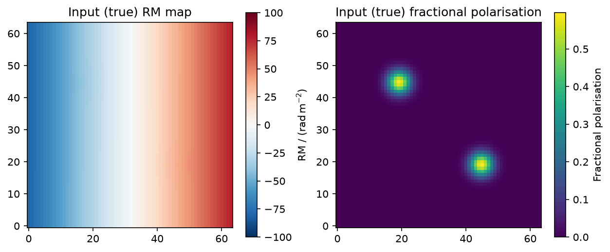
Now write Stokes Q and U to separate FITS cubes, each with a degenerate leading Stokes axis (NAXIS4 = 1).

tmpdir = Path(tempfile.mkdtemp())


def write_stokes_fits(path: Path, data: np.ndarray, stokes: int) -> None:
    header = fits.Header()
    header["CTYPE1"] = "RA---SIN"
    header["CTYPE2"] = "DEC--SIN"
    header["CTYPE3"] = "FREQ"
    header["CRVAL3"] = freq_hz[0]
    header["CDELT3"] = float(np.diff(freq_hz)[0])
    header["CRPIX3"] = 1.0
    header["CUNIT3"] = "Hz"
    header["CTYPE4"] = "STOKES"
    header["CRVAL4"] = stokes
    header["CDELT4"] = 1.0
    header["CRPIX4"] = 1.0
    fits.PrimaryHDU(data=data[np.newaxis, ...], header=header).writeto(
        path, overwrite=True
    )


stokes_q_fits = tmpdir / "cutout.q.fits"
stokes_u_fits = tmpdir / "cutout.u.fits"
write_stokes_fits(stokes_q_fits, stokes_q, stokes=2)
write_stokes_fits(stokes_u_fits, stokes_u, stokes=3)

fits.getdata(stokes_q_fits).shape

(1, 36, 64, 64)

read_fits_cube_dask reads the cube one spatial block at a time. Each block reopens the FITS file with memmap=True and slices out just that block’s rows and columns, wrapped in a dask.delayed call and assembled into a single chunked dask.array. Actual disk reads are deferred until a block is computed. The frequency axis is always kept whole in a chunk, since RM-synthesis needs every channel per pixel, and the spatial chunk size comes from a target per-chunk memory footprint. Here it is set artificially small so multiple chunks show up in this small demo cube.

In practice, peak memory during processing is a few times target_chunk_mb (roughly 2 to 4x, from buffer copies made when a block is materialised and again when it is written out), not a hard cap. It scales with chunk size, not cube size, so a target_chunk_mb set well below your available memory stays safe however large the on-disk cube is. Total RM-synthesis wall-clock time is set by the cube’s total size, not how it is chunked, so smaller chunks cost little in speed. When in doubt, prefer a smaller target_chunk_mb.

from rm_lite.utils.dask_io import read_fits_cube_dask

q_dask, q_header = read_fits_cube_dask(
    stokes_q_fits, target_chunk_mb=32 * 1024 / 1024**2
)
u_dask, _ = read_fits_cube_dask(stokes_u_fits, target_chunk_mb=32 * 1024 / 1024**2)
q_dask

Array Chunk Bytes 576.00 kiB 31.64 kiB Shape (36, 64, 64) (36, 15, 15) Dask graph 25 chunks in 81 graph layers Data type float32 numpy.ndarray

Before running RM-synthesis, estimate a robust per-channel noise directly from the cube with estimate_channel_noise_mad. It takes the MAD-based standard deviation over every pixel in each channel plane, combined across Q and U the same way compute_rmsynth_params combines a per-channel error spectrum. This feeds weight_arr below and, in the RM-CLEAN notebook, the auto-mask/threshold.

from rm_lite.utils.dask_io import estimate_channel_noise_mad

channel_noise = estimate_channel_noise_mad(q_dask, u_dask)
weight_arr = 1.0 / channel_noise**2

print(f"true per-channel noise:      {rms_noise:.4f}")
print(f"estimated per-channel noise: {channel_noise.mean():.4f}")

INFO dask_io.estimate_channel_noise_mad: Rechunking Stokes Q/U to one spatial block per channel for noise estimation.
INFO dask_io.estimate_channel_noise_mad: Per-channel noise estimation completed in 0.253 seconds.

true per-channel noise:      0.0300
estimated per-channel noise: 0.0316

Run 3D RM-synthesis with rmsynth_3d. This applies the same rmsynth_nufft/get_rmsf_nufft math used by the 1D and 2D tools across the whole cube via dask.array.map_blocks, one call per spatial chunk.

We pin phi_max_radm2/d_phi_radm2 to a small, coarse Faraday depth grid (just enough planes to cover the simulated RM range) so this demo runs quickly. A real search would use finer sampling.

from rm_lite.tools_3d.rmsynth import rmsynth_3d

help(rmsynth_3d)

Help on function rmsynth_3d in module rm_lite.tools_3d.rmsynth:

rmsynth_3d(stokes_q: 'da.Array', stokes_u: 'da.Array', freq_arr_hz: 'NDArray[np.float64]', weight_arr: 'NDArray[np.float64] | None' = None, phi_max_radm2: 'float | None' = None, d_phi_radm2: 'float | None' = None, n_samples: 'float | None' = 10.0, weight_type: "Literal['variance', 'uniform']" = 'variance', stokes_i: 'da.Array | None' = None, stokes_i_error: 'NDArray[np.float64] | da.Array | None' = None, stokes_i_model: 'da.Array | None' = None, estimate_stokes_i_noise: 'bool' = False, fit_order: 'int' = 2, fit_function: "Literal['log', 'linear']" = 'log', stokes_i_snr_cut: 'float | None' = 5.0, compute_model_error: 'bool' = False, n_error_samples: 'int' = 1000, nufft_nthreads: 'int' = 1, log_level: 'int' = 30) -> 'RMSynth3DResults'
    Run RM-synthesis on chunked Stokes Q/U cubes.

    Given a Stokes I cube or model, Q/U are divided by a per-pixel Stokes I model
    (fitted or supplied) and the FDF is rescaled to flux at the reference
    frequency; otherwise the FDF stays in Q/U flux.

    Args:
        stokes_q (da.Array): Stokes Q cube (n_freq, ny, nx), chunked spatially only.
        stokes_u (da.Array): Stokes U cube, same shape/chunks as `stokes_q`.
        freq_arr_hz (NDArray[np.float64]): Frequency array in Hz.
        weight_arr (NDArray[np.float64] | None, optional): Per-channel (not
            per-pixel) weight array. Defaults to uniform.
        phi_max_radm2 (float | None, optional): Maximum Faraday depth. Defaults to None.
        d_phi_radm2 (float | None, optional): Faraday depth resolution. Defaults to None.
        n_samples (float | None, optional): Samples across the RMSF. Defaults to 10.0.
        weight_type ("variance", "uniform", optional): Weighting. Defaults to "variance".
        stokes_i (da.Array | None, optional): Stokes I cube to fit per pixel for
            the fractional correction. Ignored if `stokes_i_model` is given.
            Defaults to None (FDF stays in Q/U flux).
        stokes_i_error (NDArray[np.float64] | da.Array | None, optional): Stokes I
            error, per-channel (n_freq,) or per-pixel cube (n_freq, ny, nx), to
            weight the fit. Defaults to None (unweighted, or estimated if
            `estimate_stokes_i_noise`).
        stokes_i_model (da.Array | None, optional): Pre-computed Stokes I model
            cube, used directly (no fitting). Takes precedence over `stokes_i`.
            Defaults to None.
        estimate_stokes_i_noise (bool, optional): Derive a per-channel error from
            `stokes_i` when no `stokes_i_error` is given. Defaults to False.
        fit_order (int, optional): Stokes I fit order; negative iterates orders and
            picks the best by AIC. Defaults to 2.
        fit_function ("log", "linear", optional): "log" = power law, "linear" =
            polynomial. Defaults to "log".
        stokes_i_snr_cut (float | None, optional): Below this frequency-averaged
            Stokes I SNR a pixel falls back to a flat model (no spectral
            correction, not blanked). None fits every pixel. Fit path only.
            Defaults to 5.0.
        compute_model_error (bool, optional): Also compute a per-pixel model error
            cube via Monte-Carlo over the fit covariance, in the same fit pass.
            Logs a warning about the compute coupling when enabled. Defaults to False.
        n_error_samples (int, optional): Monte-Carlo samples per pixel for
            `compute_model_error`. Defaults to 1000.
        nufft_nthreads (int, optional): finufft OpenMP threads per chunk. Defaults
            to 1 so dask parallelises across chunks without oversubscribing finufft's
            own threads (the fast config on many chunks). Set to 0 (finufft default,
            all cores) only when computing with few chunks on the synchronous scheduler.
        log_level (int, optional): `rm_lite` logger level while chunks run;
            defaults to WARNING to silence per-chunk noise.

    Returns:
        RMSynth3DResults: Lazy FDF cube, RMSF cube, and parameters. With a Stokes I
            model, also the model cube and the 2D reference-flux/spectral-index maps.

result = rmsynth_3d(
    q_dask,
    u_dask,
    freq_hz,
    weight_arr=weight_arr,
    phi_max_radm2=150.0,
    d_phi_radm2=10.0,
)
result.fdf_dirty_cube

Array Chunk Bytes 1.94 MiB 108.98 kiB Shape (31, 64, 64) (31, 15, 15) Dask graph 25 chunks in 165 graph layers Data type complex128 numpy.ndarray

rmsynth_3d takes dask arrays, for callers who already have Q/U loaded (e.g. from zarr). When Q/U are plain FITS files on disk, rmsynth_3d_from_fits folds the read_fits_cube_dask calls above into rmsynth_3d itself, so the two files-to-lazy-cube reads don’t need to be written out by hand each time.

from rm_lite.tools_3d.rmsynth import rmsynth_3d_from_fits

result_from_fits = rmsynth_3d_from_fits(
    stokes_q_fits,
    stokes_u_fits,
    weight_arr=weight_arr,
    phi_max_radm2=150.0,
    d_phi_radm2=10.0,
    target_chunk_mb=32 * 1024 / 1024**2,
)
np.allclose(result_from_fits.fdf_dirty_cube.compute(), result.fdf_dirty_cube.compute())

True

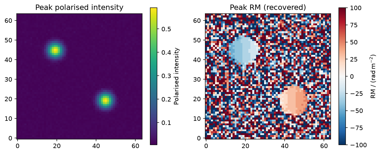
fdf_dirty_cube and rmsf_cube are still lazy; nothing has been computed yet. Let’s materialise the dirty FDF cube and look at the peak polarised intensity and recovered RM maps.

fdf_dirty_cube = result.fdf_dirty_cube.compute()
peak_pi_map = np.max(np.abs(fdf_dirty_cube), axis=0)
peak_idx_map = np.argmax(np.abs(fdf_dirty_cube), axis=0)
peak_rm_map = result.phi_arr_radm2[peak_idx_map]

fig, (ax1, ax2) = plt.subplots(1, 2, figsize=(10, 4))
im1 = ax1.imshow(peak_pi_map, origin="lower")
fig.colorbar(im1, ax=ax1, label="Polarised intensity")
ax1.set(title="Peak polarised intensity")
im2 = ax2.imshow(peak_rm_map, origin="lower", cmap="RdBu_r", vmin=-100, vmax=100)
fig.colorbar(im2, ax=ax2, label=f"RM / ({u.rad / u.m**2:latex_inline})")
ax2.set(title="Peak RM (recovered)")

[Text(0.5, 1.0, 'Peak RM (recovered)')]

Serialisation: zarr vs FITS

The dirty FDF and RMSF cubes are complex-valued, which matters for how they get written out:

• zarr supports complex128 natively, and dask.array.to_zarr writes chunk by chunk without ever materialising the full cube in memory. The write scales with chunk size, not cube size, same as the computation itself (with the same buffer-copy overhead noted above, so budget a few times target_chunk_mb, not exactly target_chunk_mb).

• FITS has no native complex dtype, and astropy.io.fits needs a full in-memory array to write. Writing an FDF cube to FITS means computing the whole cube first, then splitting it into real/imaginary (or real/imaginary/polarised-intensity) HDUs. This is the convention classic RM-Tools uses for its FDF_real_dirty.fits/FDF_im_dirty.fits/FDF_tot_dirty.fits outputs.

zarr is the better fit for cube-sized outputs; FITS remains useful for interoperability with tools that expect it.

from rm_lite.utils.dask_io import write_zarr_group

zarr_store = tmpdir / "rmsynth3d.zarr"
write_zarr_group(
    zarr_store,
    {"fdf_dirty": result.fdf_dirty_cube, "rmsf": result.rmsf_cube},
)

group = zarr.open(zarr_store)
group["fdf_dirty"].shape, group["fdf_dirty"].dtype

[########################################] | 100% Completed | 409.20 ms

INFO dask_io.write_zarr_group: Wrote ['fdf_dirty', 'rmsf'] to /tmp/tmpn_yksawa/rmsynth3d.zarr in 0.426 seconds.

((31, 64, 64), dtype('<c16'))

fits.PrimaryHDU(fdf_dirty_cube.real.astype(np.float32)).writeto(
    tmpdir / "FDF_real_dirty.fits", overwrite=True
)
fits.PrimaryHDU(fdf_dirty_cube.imag.astype(np.float32)).writeto(
    tmpdir / "FDF_im_dirty.fits", overwrite=True
)
fits.PrimaryHDU(np.abs(fdf_dirty_cube).astype(np.float32)).writeto(
    tmpdir / "FDF_tot_dirty.fits", overwrite=True
)

roundtrip = fits.getdata(tmpdir / "FDF_tot_dirty.fits")
np.allclose(roundtrip, np.abs(fdf_dirty_cube), atol=1e-5)

True

Divide out the Stokes I spectral index first on the 3D RM-synthesis with Stokes I correction page, and see the 3D RM-CLEAN page to deconvolve these dirty FDF/RMSF cubes.