2D RM-Synthesis

from __future__ import annotations

import astropy.units as u
import matplotlib.pyplot as plt
import numpy as np
from astropy.visualization import quantity_support

plt.rcParams["figure.dpi"] = 150

_ = quantity_support()
rng = np.random.default_rng(42)

Let’s set up some time-dependent spectra. We’ll vary the RM and fractional polarisation as a function of tim

freqs = np.linspace(1.1, 3.1, 128) * u.GHz
freq_hz = freqs.to(u.Hz).value
n_times = 1024
time_chan = np.arange(n_times)
rm_time = np.sin(2 * np.pi * time_chan / n_times) * 100.0
frac_pol_time = (-(np.linspace(-1, 1, n_times) ** 2) + 1) * 0.7
# psi0_time = rng.uniform(0.0, 180.0, n_times)
psi0_time = time_chan % 180

fig, (ax1, ax2, ax3) = plt.subplots(3, 1, figsize=(8, 6), sharex=True)
ax1.plot(time_chan, rm_time)
ax2.plot(time_chan, frac_pol_time)
ax3.plot(
    time_chan,
    psi0_time,
)
ax1.set(
    ylabel=f"RM / ({u.rad / u.m**2:latex_inline})",
    title="Input data for RM synthesis",
)
ax2.set(
    ylabel="Fractional Polarisation",
)

ax3.set(
    xlabel="Time Channel",
    ylabel="Polaristion angle / deg",
)

[Text(0.5, 0, 'Time Channel'), Text(0, 0.5, 'Polaristion angle / deg')]

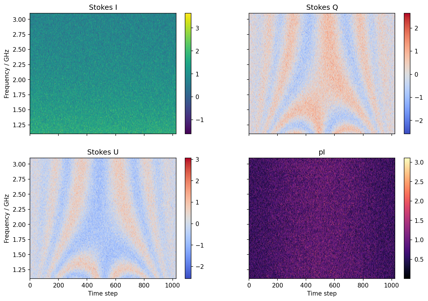
Now we’ll simulate the spectra and place in a 2D array

from rm_lite.utils.fitting import power_law
from rm_lite.utils.synthesis import faraday_simple_spectrum, freq_to_lambda2

dynamic_spectrum = np.empty((len(freqs), n_times), dtype=np.complex128)
total_dynamic_spectrum = np.empty((len(freqs), n_times), dtype=np.float64)


for time_step, (rm_radm2, frac_pol, psi0_deg) in enumerate(
    zip(rm_time, frac_pol_time, psi0_time)
):
    complex_data_noiseless = faraday_simple_spectrum(
        freq_hz,
        frac_pol=frac_pol,
        psi0_deg=psi0_deg,
        rm_radm2=rm_radm2,
    )
    stokes_i_flux = 1.0
    spectral_index = -0.7
    rms_noise = 0.5

    stokes_i_model = power_law(order=1)
    stokes_i_noiseless = stokes_i_model(
        freq_hz / (np.mean(freq_hz)), stokes_i_flux, spectral_index
    )
    stokes_i_noise = rng.normal(0, rms_noise, size=freq_hz.size)
    stokes_i_noisy = stokes_i_noiseless + stokes_i_noise

    stokes_q_noise = rng.normal(0, rms_noise, size=freq_hz.size)
    stokes_u_noise = rng.normal(0, rms_noise, size=freq_hz.size)
    complex_noise = stokes_q_noise + 1j * stokes_u_noise

    complex_flux = complex_data_noiseless * stokes_i_noiseless
    complex_data_noisy = complex_data_noiseless + complex_noise

    dynamic_spectrum[:, time_step] = complex_data_noisy
    total_dynamic_spectrum[:, time_step] = stokes_i_noisy

fig, axs = plt.subplots(2, 2, figsize=(12, 8), sharex=True, sharey=True)
ax1, ax2, ax3, ax4 = axs.flatten()

im = ax1.imshow(
    total_dynamic_spectrum,
    aspect="auto",
    origin="lower",
    extent=(0, n_times, np.min(freqs), np.max(freqs)),
)
fig.colorbar(im, ax=ax1)
ax1.set(ylabel="Frequency / GHz", title="Stokes I")

im = ax2.imshow(
    np.real(dynamic_spectrum),
    aspect="auto",
    origin="lower",
    extent=(0, n_times, np.min(freqs), np.max(freqs)),
    cmap="coolwarm",
)
ax2.set(
    title="Stokes Q",
)
fig.colorbar(im, ax=ax2)

im = ax3.imshow(
    np.imag(dynamic_spectrum),
    aspect="auto",
    origin="lower",
    extent=(0, n_times, np.min(freqs), np.max(freqs)),
    cmap="coolwarm",
)
ax3.set(
    title="Stokes U",
    xlabel="Time step",
    ylabel="Frequency / GHz",
)
fig.colorbar(im, ax=ax3)

im = ax4.imshow(
    np.abs(dynamic_spectrum),
    aspect="auto",
    origin="lower",
    extent=(0, n_times, np.min(freqs), np.max(freqs)),
    cmap="magma",
)
fig.colorbar(im, ax=ax4)
ax4.set(
    xlabel="Time step",
    title="pI",
)

[Text(0.5, 0, 'Time step'), Text(0.5, 1.0, 'pI')]

To do the RM synthesis, we’ll use some of the utility functions directly

from rm_lite.utils.synthesis import make_phi_arr, rmsynth_nufft

help(rmsynth_nufft)
help(make_phi_arr)

Help on function rmsynth_nufft in module rm_lite.utils.synthesis:

rmsynth_nufft(complex_pol_arr: 'NDArray[np.complex128]', lambda_sq_arr_m2: 'NDArray[np.float64]', phi_arr_radm2: 'NDArray[np.float64]', weight_arr: 'NDArray[np.float64]', lam_sq_0_m2: 'float', eps: 'float' = 1e-06) -> 'NDArray[np.complex128]'
    Run RM-synthesis on a cube of Stokes Q and U data using the NUFFT method.

    Args:
        complex_pol_arr (NDArray[np.complex128]): Complex polarisation values (Q + iU)
        lambda_sq_arr_m2 (NDArray[np.float64]): Wavelength^2 values in m^2
        phi_arr_radm2 (NDArray[np.float64]): Faraday depth values in rad/m^2
        weight_arr (NDArray[np.float64]): Weight array
        lam_sq_0_m2 (Optional[float], optional): Reference wavelength^2 in m^2. Defaults to None.
        eps (float, optional): NUFFT tolerance. Defaults to 1e-6.

    Raises:
        ValueError: If the weight and lambda^2 arrays are not the same shape.
        ValueError: If the Stokes Q and U data arrays are not the same shape.
        ValueError: If the data dimensions are > 3.
        ValueError: If the data depth does not match the lambda^2 vector.

    Returns:
        NDArray[np.float64]: Dirty Faraday dispersion function cube

Help on function make_phi_arr in module rm_lite.utils.synthesis:

make_phi_arr(phi_max_radm2: 'float', d_phi_radm2: 'float') -> 'NDArray[np.float64]'
    Construct a Faraday depth array.

    Args:
        phi_max_radm2 (float): Maximum Faraday depth in rad/m^2
        d_phi_radm2 (float): Spacing in Faraday depth in rad/m^2

    Returns:
        NDArray[np.float64]: Faraday depth array in rad/m^2

phis = make_phi_arr(500, 0.1)
lam_sq_0_m2 = float(np.mean(freq_to_lambda2(freq_hz)))

fdf_spectrum = rmsynth_nufft(
    complex_pol_arr=dynamic_spectrum,
    lambda_sq_arr_m2=freq_to_lambda2(freq_hz),
    phi_arr_radm2=phis,
    weight_arr=np.ones_like(freq_hz),
    lam_sq_0_m2=lam_sq_0_m2,
)

INFO synthesis.rmsynth_nufft: Running RM-synthesis using the NUFFTs over 10001 Faraday depth channels.
INFO synthesis.rmsynth_nufft: NUFFT complete in 0.185 seconds.

Let’s look at the results

fig, ax = plt.subplots()
ax.imshow(
    np.abs(fdf_spectrum),
    # aspect="auto",
    origin="lower",
    extent=(0, n_times, np.min(phis), np.max(phis)),
)
ax.set(
    xlabel="Time step",
    ylabel=f"Faraday depth / ({u.rad / u.m**2:latex_inline})",
    title="Dynamic spectrum",
)

[Text(0.5, 0, 'Time step'),
 Text(0, 0.5, 'Faraday depth / ($\\mathrm{rad\\,m^{-2}}$)'),
 Text(0.5, 1.0, 'Dynamic spectrum')]

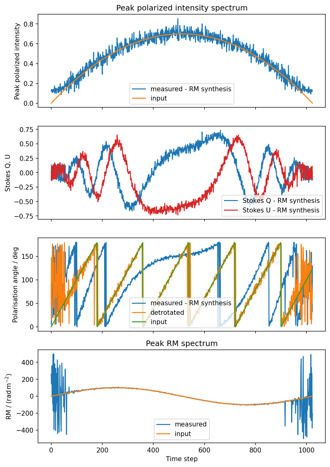
Now let’s recover the PI and RM from the Faraday spectrum. Taking the mean will not perform well due to bandwidth depolarisation, but RM-sythnesis gives us the full-bandwidth sensitivity with a coherent sum.

Note that at low SNR Ricean bias becomes significant. Further, our uncertainty in RM also goes up.

peak_pi_spectrum = np.max(np.abs(fdf_spectrum), axis=0)

max_pixels = np.argmax(np.abs(fdf_spectrum), axis=0)

peak_rm_spectrum = phis[max_pixels]
peak_q_spectrum = np.real(fdf_spectrum)[max_pixels, np.arange(fdf_spectrum.shape[1])]
peak_u_spectrum = np.imag(fdf_spectrum)[max_pixels, np.arange(fdf_spectrum.shape[1])]
peak_pa_spectrum = np.rad2deg(0.5 * np.arctan2(peak_u_spectrum, peak_q_spectrum)) % 180
peak_pa_spectrum_detrot = (
    np.rad2deg(np.deg2rad(peak_pa_spectrum) - (peak_rm_spectrum * lam_sq_0_m2)) % 180
)


fig, (ax1, ax2, ax3, ax4) = plt.subplots(4, 1, sharex=True, figsize=(8, 12))
ax1.plot(time_chan, peak_pi_spectrum, label="measured - RM synthesis")
ax1.plot(time_chan, frac_pol_time, label="input")

ax2.plot(
    time_chan,
    peak_q_spectrum,
    c="tab:blue",
    label="Stokes Q - RM synthesis",
)
ax2.plot(
    time_chan,
    peak_u_spectrum,
    c="tab:red",
    label="Stokes U - RM synthesis",
)
ax2.set(
    ylabel="Stokes Q, U",
)
ax2.legend()

ax3.plot(
    time_chan,
    peak_pa_spectrum,
    label="measured - RM synthesis",
)
ax3.plot(
    time_chan,
    peak_pa_spectrum_detrot,
    label="detrotated",
)
ax3.plot(
    time_chan,
    psi0_time,
    label="input",
)
ax3.legend()
ax3.set(
    ylabel="Polarisation angle / deg",
)

ax1.legend()

ax4.plot(time_chan, peak_rm_spectrum, label="measured")
ax4.plot(time_chan, rm_time, label="input")
ax4.legend()

ax4.set(
    xlabel="Time step",
    ylabel=f"RM / ({u.rad / u.m**2:latex_inline})",
    title="Peak RM spectrum",
)
ax1.set(
    ylabel="Peak polarized intensity",
    title="Peak polarized intensity spectrum",
)

[Text(0, 0.5, 'Peak polarized intensity'),
 Text(0.5, 1.0, 'Peak polarized intensity spectrum')]