1D RM-CLEAN
[1]:
from __future__ import annotations

import astropy.units as u
import matplotlib.pyplot as plt
import numpy as np
from astropy.visualization import quantity_support
from rm_lite.tools_1d import rmclean, rmsynth

plt.rcParams["figure.dpi"] = 150

_ = quantity_support()
rng = np.random.default_rng(42)
First, we’ll start with the same data s the 1D RM-synth example. Keeping it simple, we’ll use a Faraday simple source with a bit of noise.
I’ll skip the details here, see the RM-synth page for more info.
[2]:
from rm_lite.utils.fitting import power_law
from rm_lite.utils.simulate import faraday_simple_spectrum, faraday_slab_spectrum
from rm_lite.utils.synthesis import freq_to_lambda2

bw_low = 288
bw_mid = 144
bw_high = 288
low = np.linspace(943.5 - bw_low / 2, 943.5 + bw_low / 2, 36) * u.MHz
mid = np.linspace(1367.5 - bw_mid / 2, 1367.5 + bw_mid / 2, 9) * u.MHz
high = np.linspace(1655.5 - bw_high / 2, 1655.5 + bw_high / 2, 9) * u.MHz
freqs = np.concatenate([low, mid, high])
freq_hz = freqs.to(u.Hz).value

delta_rm_radm2 = 30
rm_radm2 = 100
frac_pol = 0.7
psi0_deg = 10

complex_data_noiseless = faraday_simple_spectrum(
    freq_to_lambda2(freq_hz),
    frac_pol=frac_pol,
    psi0_deg=psi0_deg,
    rm_radm2=rm_radm2,
)
stokes_i_flux = 2.0
spectral_index = -0.7
rms_noise = 0.1

stokes_i_model = power_law(order=1)
stokes_i_noiseless = stokes_i_model(
    freq_hz / (np.mean(freq_hz)), stokes_i_flux, spectral_index
)
stokes_i_noise = rng.normal(0, rms_noise, size=freq_hz.size)
stokes_i_noisy = stokes_i_noiseless + stokes_i_noise


stokes_q_noise = rng.normal(0, rms_noise, size=freq_hz.size)
stokes_u_noise = rng.normal(0, rms_noise, size=freq_hz.size)
complex_noise = stokes_q_noise + 1j * stokes_u_noise

complex_flux = complex_data_noiseless * stokes_i_noiseless
complex_data_noisy = complex_data_noiseless + complex_noise
rm_syth_results = rmsynth.run_rmsynth(
    freq_arr_hz=freq_hz,
    complex_pol_arr=complex_data_noisy,
    complex_pol_error=np.ones_like(complex_data_noiseless) * rms_noise,
    do_fit_rmsf=True,
    n_samples=100,
)
WARNING rmsynth.run_rmsynth: Stokes I array/errors or model not provided. No fractional polarization will be calculated.
INFO synthesis.rmsynth_nufft: Running RM-synthesis using the NUFFTs over 2001 Faraday depth channels.
INFO synthesis.rmsynth_nufft: NUFFT complete in 0.00456 seconds.
INFO synthesis.get_rmsf_nufft: Fitting main lobe in each RMSF spectrum.
INFO rmsynth._run_rmsynth: RM-synthesis completed in 14.18ms.
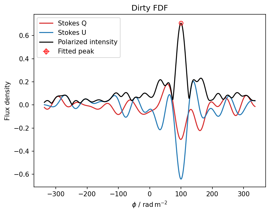
Let’s remind ourselves of the what the dirty spectrum looks like
[3]:
fdf_parameters, fdf_arrs, rmsf_arrs, stokes_i_arrs = rm_syth_results

phi_arr_radm2 = fdf_arrs["phi_arr_radm2"].to_numpy()
fdf_dirty_arr = fdf_arrs["fdf_dirty_complex_arr"].to_numpy().astype(complex)

fig, ax = plt.subplots()

ax.plot(
    phi_arr_radm2,
    fdf_dirty_arr.real,
    color="tab:red",
    label="Stokes Q",
)
ax.plot(
    phi_arr_radm2,
    fdf_dirty_arr.imag,
    color="tab:blue",
    label="Stokes U",
)
ax.plot(
    phi_arr_radm2,
    np.abs(fdf_dirty_arr),
    color="k",
    label="Polarized intensity",
)

ax.errorbar(
    fdf_parameters["peak_rm_fit"],
    fdf_parameters["peak_pi_fit"],
    xerr=fdf_parameters["peak_rm_fit_error"],
    yerr=fdf_parameters["peak_pi_error"],
    fmt="o",
    lw=1,
    color="red",
    mfc="none",
    label="Fitted peak",
)

ax.set(
    xlabel=rf"$\phi$ / {u.rad / u.m**2:latex_inline}",
    ylabel="Flux density",
    title="Dirty FDF",
)
ax.legend()
[3]:
<matplotlib.legend.Legend at 0x74afefbee480>
We can use the convenience function rmclean.run_rmclean_from_synth to directly take the outputs of 1D RM-synthesis for RM-CLEAN.
Inspired by WSClean, rm_lite implements a deep cleaning mode with auto-masking and auto-thresholding based on the noise profile.
[4]:
help(rmclean.run_rmclean_from_synth)
Help on function run_rmclean_from_synth in module rm_lite.tools_1d.rmclean:

run_rmclean_from_synth(rm_synth_1d_results: 'RMSynth1DResults', auto_mask: 'float' = 7, auto_threshold: 'float' = 1, max_iter: 'int' = 100000, gain: 'float' = 0.1, mask_arr: 'NDArray[np.bool_] | None' = None, moment_threshold_snr: 'float' = 5.0, multiscale: 'bool' = False, multiscale_scales: 'NDArray[np.float64] | None' = None, multiscale_n_scales: 'int | None' = None, multiscale_kernel: "Literal['tapered_quad', 'gaussian']" = 'tapered_quad', multiscale_max_iter_sub_minor: 'int' = 10000, multiscale_sub_minor_fraction: 'float' = 0.5, multiscale_selection_margin: 'float' = 0.08) -> 'RMClean1DResults'
    Run RM-CLEAN on the results of RM-synth.

    Args:
        rm_synth_1d_results (RMSynth1DResults): Results from RM-synth.
        auto_mask (float, optional): Masking threshold in SNR. Defaults to 7.
        auto_threshold (float, optional): Cleaning threshold in SNR. Defaults to 1.
        max_iter (int, optional): Maximum CLEAN iterations. Defaults to 10_000.
        gain (float, optional): CLEAN gain. Defaults to 0.1.
        mask_arr (NDArray[np.bool_] | None, optional): Optional mask array. Defaults to None.
        moment_threshold_snr (float, optional): SNR cut (times the theoretical FDF noise) applied to the clean FDF amplitudes before computing the Faraday moments. Defaults to 5.0.
        multiscale (bool, optional): Use multiscale RM-CLEAN (recovers Faraday-thick structure). Defaults to False.
        multiscale_scales (NDArray[np.float64] | None, optional): Explicit scales (RMSF FWHM units); None auto-selects from the RMSF max scale.
        multiscale_n_scales (int | None, optional): Cap on the auto scale count.
        multiscale_kernel ("tapered_quad" | "gaussian", optional): Scale kernel. Defaults to "tapered_quad".
        multiscale_max_iter_sub_minor (int, optional): Max sub-minor iterations per scale. Defaults to 10_000.
        multiscale_sub_minor_fraction (float, optional): Sub-minor re-selection fraction. Defaults to 0.5.
        multiscale_selection_margin (float, optional): Hybrid scale-selection parsimony margin in [0, 1). Among scales within this fraction of the best matched-filter score the smallest is chosen, keeping points on the delta scale. Defaults to 0.08.

    Returns:
        RMClean1DResults: RM-CLEAN results: `fdf_parameters`, `fdf_arrs`, `clean_parameters`.
[5]:
rmclean_results = rmclean.run_rmclean_from_synth(
    rm_synth_1d_results=rm_syth_results, auto_mask=10, auto_threshold=0.5
)
INFO rmclean.run_rmclean_from_synth: Theoretical noise: TheoreticalNoise(fdf_error_noise=0.006804138174397718, fdf_q_noise=0.013608276348795436, fdf_u_noise=0.0)
INFO rmclean.run_rmclean_from_synth: Auto mask: 0.07, Auto threshold: 0.00, Max iterations: 100000, Gain: 0.1
INFO clean.minor_cycle: Starting initial minor loop...
INFO clean.minor_loop: Starting minor loop... 1 pixels in the mask
INFO clean.minor_loop: Threshold reached. Exiting loop...performed 51 iterations
INFO clean.minor_cycle: Initial loop complete. Starting deep clean...
INFO clean.minor_loop: Starting minor loop... 3 pixels in the mask
INFO clean.minor_loop: Threshold reached. Exiting loop...performed 51 iterations
[6]:
rmclean_results
[6]:
RMClean1DResults(fdf_parameters=shape: (1, 36)
┌───────────┬───────────┬───────────┬───────────┬───┬───────────┬───────────┬───────────┬──────────┐
│ fdf_error ┆ peak_pi_f ┆ peak_pi_e ┆ peak_pi_f ┆ … ┆ mom0_debi ┆ mom1_radm ┆ mom2_radm ┆ moment_t │
│ _mad      ┆ it        ┆ rror      ┆ it_debias ┆   ┆ as        ┆ 2         ┆ 2         ┆ hreshold │
│ ---       ┆ ---       ┆ ---       ┆ ---       ┆   ┆ ---       ┆ ---       ┆ ---       ┆ _snr     │
│ f64       ┆ f64       ┆ f64       ┆ f64       ┆   ┆ f64       ┆ f64       ┆ f64       ┆ ---      │
│           ┆           ┆           ┆           ┆   ┆           ┆           ┆           ┆ f64      │
╞═══════════╪═══════════╪═══════════╪═══════════╪═══╪═══════════╪═══════════╪═══════════╪══════════╡
│ NaN       ┆ 0.707165  ┆ 0.006804  ┆ 0.70709   ┆ … ┆ 0.721711  ┆ 94.914026 ┆ 50.991387 ┆ 5.0      │
└───────────┴───────────┴───────────┴───────────┴───┴───────────┴───────────┴───────────┴──────────┘, fdf_arrs=shape: (2_001, 5)
┌───────────────┬────────────────────┬────────────────────┬────────────────────┬───────────────────┐
│ phi_arr_radm2 ┆ fdf_dirty_complex_ ┆ fdf_clean_complex_ ┆ fdf_model_complex_ ┆ fdf_residual_comp │
│ ---           ┆ arr                ┆ arr                ┆ arr                ┆ lex_arr           │
│ f64           ┆ ---                ┆ ---                ┆ ---                ┆ ---               │
│               ┆ object             ┆ object             ┆ object             ┆ object            │
╞═══════════════╪════════════════════╪════════════════════╪════════════════════╪═══════════════════╡
│ -336.725921   ┆ (-0.02201829946284 ┆ (-0.00396336358318 ┆ 0j                 ┆ (-0.0039633635831 │
│               ┆ 6964+0.00164…      ┆ 2648-0.00653…      ┆                    ┆ 82648-0.00653…    │
│ -336.389195   ┆ (-0.02299621077262 ┆ (-0.00402671441356 ┆ 0j                 ┆ (-0.0040267144135 │
│               ┆ 284+0.001460…      ┆ 98665-0.0062…      ┆                    ┆ 698665-0.0062…    │
│ -336.052469   ┆ (-0.02395216902624 ┆ (-0.00408727466314 ┆ 0j                 ┆ (-0.0040872746631 │
│               ┆ 6483+0.00127…      ┆ 5158-0.00584…      ┆                    ┆ 45158-0.00584…    │
│ -335.715743   ┆ (-0.02488486436654 ┆ (-0.00414499270432 ┆ 0j                 ┆ (-0.0041449927043 │
│               ┆ 0808+0.00108…      ┆ 459-0.005480…      ┆                    ┆ 2459-0.005480…    │
│ -335.379017   ┆ (-0.02579299105138 ┆ (-0.00419980648441 ┆ 0j                 ┆ (-0.0041998064844 │
│               ┆ 939+0.000899…      ┆ 9988-0.00510…      ┆                    ┆ 19988-0.00510…    │
│ …             ┆ …                  ┆ …                  ┆ …                  ┆ …                 │
│ 335.379017    ┆ (-0.01154276638529 ┆ (-0.01048165184254 ┆ 0j                 ┆ (-0.0104816518425 │
│               ┆ 7472+0.03547…      ┆ 5747+0.02410…      ┆                    ┆ 45747+0.02410…    │
│ 335.715743    ┆ (-0.01216991132307 ┆ (-0.01102357839809 ┆ 0j                 ┆ (-0.0110235783980 │
│               ┆ 7836+0.03526…      ┆ 4619+0.02413…      ┆                    ┆ 94619+0.02413…    │
│ 336.052469    ┆ (-0.01275387931273 ┆ (-0.01156767057117 ┆ 0j                 ┆ (-0.0115676705711 │
│               ┆ 7802+0.03504…      ┆ 244+0.024156…      ┆                    ┆ 7244+0.024156…    │
│ 336.389195    ┆ (-0.01329469655533 ┆ (-0.01211333882233 ┆ 0j                 ┆ (-0.0121133388223 │
│               ┆ 1541+0.03483…      ┆ 2934+0.02417…      ┆                    ┆ 32934+0.02417…    │
│ 336.725921    ┆ (-0.01379245060858 ┆ (-0.01265997956029 ┆ 0j                 ┆ (-0.0126599795602 │
│               ┆ 4375+0.03461…      ┆ 987+0.024189…      ┆                    ┆ 9987+0.024189…    │
└───────────────┴────────────────────┴────────────────────┴────────────────────┴───────────────────┘, clean_parameters=shape: (1, 4)
┌──────────┬───────────┬────────┬──────────────────┐
│ mask     ┆ threshold ┆ n_iter ┆ n_sub_minor_iter │
│ ---      ┆ ---       ┆ ---    ┆ ---              │
│ f64      ┆ f64       ┆ i64    ┆ i64              │
╞══════════╪═══════════╪════════╪══════════════════╡
│ 0.068041 ┆ 0.003402  ┆ 51     ┆ 51               │
└──────────┴───────────┴────────┴──────────────────┘)
[7]:
# Extract the DataFrames
clean_arrs = rmclean_results.fdf_arrs
clean_fdf_params = rmclean_results.fdf_parameters
clean_params = rmclean_results.clean_parameters
[8]:
# Extract some arrays
phi_arr_radm2 = clean_arrs["phi_arr_radm2"].to_numpy()
fdf_dirty_arr = clean_arrs["fdf_dirty_complex_arr"].to_numpy().astype(complex)
fdf_clean_arr = clean_arrs["fdf_clean_complex_arr"].to_numpy().astype(complex)
fdf_model_arr = clean_arrs["fdf_model_complex_arr"].to_numpy().astype(complex)
fdf_residual_arr = clean_arrs["fdf_residual_complex_arr"].to_numpy().astype(complex)
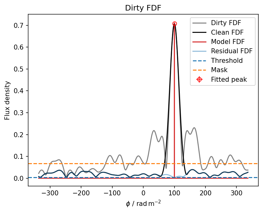
Let’s look at how the CLEAN went. Note that the deep clean allows us to model the entire simple component.
[9]:
fig, ax = plt.subplots()

ax.plot(
    phi_arr_radm2,
    np.abs(fdf_dirty_arr),
    color="k",
    label="Dirty FDF",
    alpha=0.5,
)
ax.plot(
    phi_arr_radm2,
    np.abs(fdf_clean_arr),
    color="k",
    label="Clean FDF",
)
ax.step(
    phi_arr_radm2,
    np.abs(fdf_model_arr),
    color="tab:red",
    label="Model FDF",
    where="mid",
)
ax.plot(
    phi_arr_radm2,
    np.abs(fdf_residual_arr),
    color="tab:blue",
    label="Residual FDF",
    alpha=0.5,
)

ax.errorbar(
    clean_fdf_params["peak_rm_fit"],
    clean_fdf_params["peak_pi_fit"],
    xerr=clean_fdf_params["peak_rm_fit_error"],
    yerr=clean_fdf_params["peak_pi_error"],
    fmt="o",
    lw=1,
    color="red",
    mfc="none",
    label="Fitted peak",
)

ax.axhline(
    y=clean_params["threshold"][0],
    color="tab:blue",
    label="Threshold",
    linestyle="--",
)
ax.axhline(
    y=clean_params["mask"][0],
    color="tab:orange",
    label="Mask",
    linestyle="--",
)

ax.set(
    xlabel=rf"$\phi$ / {u.rad / u.m**2:latex_inline}",
    ylabel="Flux density",
    title="Dirty FDF",
)
ax.legend()
[9]:
<matplotlib.legend.Legend at 0x74afec5109e0>
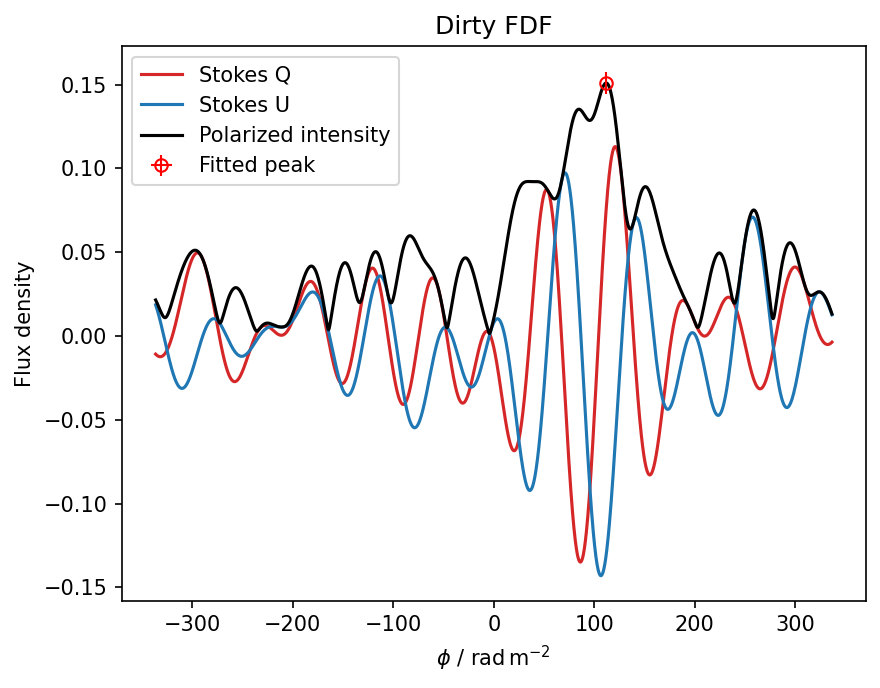
Now let’s take a look at the more complex example.
[10]:
delta_rm_radm2 = 30
rm_radm2 = 100
frac_pol = 0.5
psi0_deg = 10
complex_data_noiseless = faraday_slab_spectrum(
    freq_to_lambda2(freq_hz),
    frac_pol=frac_pol,
    psi0_deg=psi0_deg,
    rm_radm2=rm_radm2,
    delta_rm_radm2=delta_rm_radm2,
)


stokes_i_flux = 1.0
spectral_index = -0.7
rms_noise = 0.1


stokes_i_model = power_law(order=1)
stokes_i_noiseless = stokes_i_model(
    freq_hz / (np.mean(freq_hz)), stokes_i_flux, spectral_index
)
stokes_i_noise = rng.normal(0, rms_noise, size=freq_hz.size)
stokes_i_noisy = stokes_i_noiseless + stokes_i_noise


stokes_q_noise = rng.normal(0, rms_noise, size=freq_hz.size)
stokes_u_noise = rng.normal(0, rms_noise, size=freq_hz.size)
complex_noise = stokes_q_noise + 1j * stokes_u_noise

complex_flux = complex_data_noiseless * stokes_i_noiseless
complex_data_noisy = complex_data_noiseless + complex_noise
[11]:
rm_syth_results = rmsynth.run_rmsynth(
    freq_arr_hz=freq_hz,
    complex_pol_arr=complex_data_noisy,
    complex_pol_error=np.ones_like(complex_data_noiseless) * rms_noise,
    do_fit_rmsf=True,
    n_samples=100,
)
WARNING rmsynth.run_rmsynth: Stokes I array/errors or model not provided. No fractional polarization will be calculated.
INFO synthesis.rmsynth_nufft: Running RM-synthesis using the NUFFTs over 2001 Faraday depth channels.
INFO synthesis.rmsynth_nufft: NUFFT complete in 0.00248 seconds.
INFO synthesis.get_rmsf_nufft: Fitting main lobe in each RMSF spectrum.
INFO rmsynth._run_rmsynth: RM-synthesis completed in 8.17ms.
[12]:
fdf_parameters, fdf_arrs, rmsf_arrs, stokes_i_arrs = rm_syth_results

phi_arr_radm2 = fdf_arrs["phi_arr_radm2"].to_numpy()
fdf_dirty_arr = fdf_arrs["fdf_dirty_complex_arr"].to_numpy().astype(complex)

fig, ax = plt.subplots()

ax.plot(
    phi_arr_radm2,
    fdf_dirty_arr.real,
    color="tab:red",
    label="Stokes Q",
)
ax.plot(
    phi_arr_radm2,
    fdf_dirty_arr.imag,
    color="tab:blue",
    label="Stokes U",
)
ax.plot(
    phi_arr_radm2,
    np.abs(fdf_dirty_arr),
    color="k",
    label="Polarized intensity",
)

ax.errorbar(
    fdf_parameters["peak_rm_fit"],
    fdf_parameters["peak_pi_fit"],
    xerr=fdf_parameters["peak_rm_fit_error"],
    yerr=fdf_parameters["peak_pi_error"],
    fmt="o",
    lw=1,
    color="red",
    mfc="none",
    label="Fitted peak",
)

ax.set(
    xlabel=rf"$\phi$ / {u.rad / u.m**2:latex_inline}",
    ylabel="Flux density",
    title="Dirty FDF",
)
ax.legend()
[12]:
<matplotlib.legend.Legend at 0x74b0207737d0>
[13]:
rmclean_results = rmclean.run_rmclean_from_synth(
    rm_synth_1d_results=rm_syth_results, auto_mask=10, auto_threshold=0.5
)

clean_arrs = rmclean_results.fdf_arrs
clean_fdf_params = rmclean_results.fdf_parameters
clean_params = rmclean_results.clean_parameters


phi_arr_radm2 = clean_arrs["phi_arr_radm2"].to_numpy()
fdf_dirty_arr = clean_arrs["fdf_dirty_complex_arr"].to_numpy().astype(complex)
fdf_clean_arr = clean_arrs["fdf_clean_complex_arr"].to_numpy().astype(complex)
fdf_model_arr = clean_arrs["fdf_model_complex_arr"].to_numpy().astype(complex)
fdf_residual_arr = clean_arrs["fdf_residual_complex_arr"].to_numpy().astype(complex)
INFO rmclean.run_rmclean_from_synth: Theoretical noise: TheoreticalNoise(fdf_error_noise=0.006804138174397718, fdf_q_noise=0.013608276348795436, fdf_u_noise=0.0)
INFO rmclean.run_rmclean_from_synth: Auto mask: 0.07, Auto threshold: 0.00, Max iterations: 100000, Gain: 0.1
INFO clean.minor_cycle: Starting initial minor loop...
INFO clean.minor_loop: Starting minor loop... 1 pixels in the mask
INFO clean.minor_loop: Threshold reached. Exiting loop...performed 101 iterations
INFO clean.minor_cycle: Initial loop complete. Starting deep clean...
INFO clean.minor_loop: Starting minor loop... 2 pixels in the mask
INFO clean.minor_loop: Threshold reached. Exiting loop...performed 101 iterations
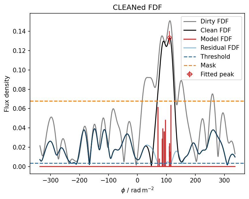
[14]:
fig, ax = plt.subplots()

ax.plot(
    phi_arr_radm2,
    np.abs(fdf_dirty_arr),
    color="k",
    label="Dirty FDF",
    alpha=0.5,
)
ax.plot(
    phi_arr_radm2,
    np.abs(fdf_clean_arr),
    color="k",
    label="Clean FDF",
)
ax.step(
    phi_arr_radm2,
    np.abs(fdf_model_arr),
    color="tab:red",
    label="Model FDF",
    where="mid",
)
ax.plot(
    phi_arr_radm2,
    np.abs(fdf_residual_arr),
    color="tab:blue",
    label="Residual FDF",
    alpha=0.5,
)

ax.errorbar(
    clean_fdf_params["peak_rm_fit"],
    clean_fdf_params["peak_pi_fit"],
    xerr=clean_fdf_params["peak_rm_fit_error"],
    yerr=clean_fdf_params["peak_pi_error"],
    fmt="o",
    lw=1,
    color="red",
    mfc="none",
    label="Fitted peak",
)
ax.axhline(
    y=clean_params["threshold"][0],
    color="tab:blue",
    label="Threshold",
    linestyle="--",
)
ax.axhline(
    y=clean_params["mask"][0],
    color="tab:orange",
    label="Mask",
    linestyle="--",
)

ax.set(
    xlabel=rf"$\phi$ / {u.rad / u.m**2:latex_inline}",
    ylabel="Flux density",
    title="CLEANed FDF",
)
ax.legend()
[14]:
<matplotlib.legend.Legend at 0x74afec11ef90>
[ ]: