2D RM-Synthesis

from __future__ import annotations

import astropy.units as u
import matplotlib.pyplot as plt
import numpy as np
from astropy.visualization import quantity_support

plt.rcParams["figure.dpi"] = 150

_ = quantity_support()
rng = np.random.default_rng(42)

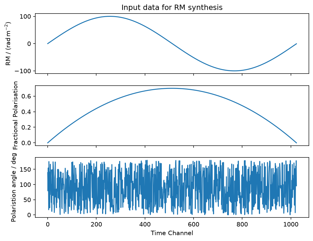
Let’s set up some time-dependent spectra. We’ll vary the RM and fractional polarisation as a function of tim

freqs = np.linspace(1.1, 3.1, 128) * u.GHz
freq_hz = freqs.to(u.Hz).value
n_times = 1024
time_chan = np.arange(n_times)
rm_time = np.sin(2 * np.pi * time_chan / n_times) * 100.0
frac_pol_time = (-(np.linspace(-1, 1, n_times) ** 2) + 1) * 0.7
psi0_time = rng.uniform(0.0, 180.0, n_times)

fig, (ax1, ax2, ax3) = plt.subplots(3, 1, figsize=(8, 6), sharex=True)
ax1.plot(time_chan, rm_time)
ax2.plot(time_chan, frac_pol_time)
ax3.plot(
    time_chan,
    psi0_time,
)
ax1.set(
    ylabel=f"RM / ({u.rad / u.m**2:latex_inline})",
    title="Input data for RM synthesis",
)
ax2.set(
    ylabel="Fractional Polarisation",
)

ax3.set(
    xlabel="Time Channel",
    ylabel="Polaristion angle / deg",
)

[Text(0.5, 0, 'Time Channel'), Text(0, 0.5, 'Polaristion angle / deg')]

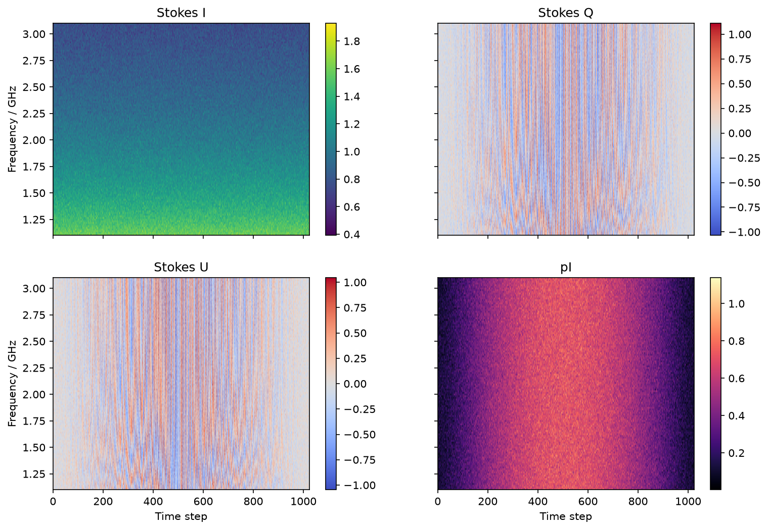
Now we’ll simulate the spectra and place in a 2D array

from rm_lite.utils.fitting import power_law
from rm_lite.utils.synthesis import faraday_simple_spectrum, freq_to_lambda2

dynamic_spectrum = np.empty((len(freqs), n_times), dtype=np.complex128)
total_dynamic_spectrum = np.empty((len(freqs), n_times), dtype=np.float64)


for time_step, (rm_radm2, frac_pol, psi0_deg) in enumerate(
    zip(rm_time, frac_pol_time, psi0_time, strict=False)
):
    complex_data_noiseless = faraday_simple_spectrum(
        freq_hz,
        frac_pol=frac_pol,
        psi0_deg=psi0_deg,
        rm_radm2=rm_radm2,
    )
    stokes_i_flux = 1.0
    spectral_index = -0.7
    rms_noise = 0.1

    stokes_i_model = power_law(order=1)
    stokes_i_noiseless = stokes_i_model(
        freq_hz / (np.mean(freq_hz)), stokes_i_flux, spectral_index
    )
    stokes_i_noise = rng.normal(0, rms_noise, size=freq_hz.size)
    stokes_i_noisy = stokes_i_noiseless + stokes_i_noise

    stokes_q_noise = rng.normal(0, rms_noise, size=freq_hz.size)
    stokes_u_noise = rng.normal(0, rms_noise, size=freq_hz.size)
    complex_noise = stokes_q_noise + 1j * stokes_u_noise

    complex_flux = complex_data_noiseless * stokes_i_noiseless
    complex_data_noisy = complex_data_noiseless + complex_noise

    dynamic_spectrum[:, time_step] = complex_data_noisy
    total_dynamic_spectrum[:, time_step] = stokes_i_noisy

fig, axs = plt.subplots(2, 2, figsize=(12, 8), sharex=True, sharey=True)
ax1, ax2, ax3, ax4 = axs.flatten()

im = ax1.imshow(
    total_dynamic_spectrum,
    aspect="auto",
    origin="lower",
    extent=(0, n_times, np.min(freqs), np.max(freqs)),
)
fig.colorbar(im, ax=ax1)
ax1.set(ylabel="Frequency / GHz", title="Stokes I")

im = ax2.imshow(
    np.real(dynamic_spectrum),
    aspect="auto",
    origin="lower",
    extent=(0, n_times, np.min(freqs), np.max(freqs)),
    cmap="coolwarm",
)
ax2.set(
    title="Stokes Q",
)
fig.colorbar(im, ax=ax2)

im = ax3.imshow(
    np.imag(dynamic_spectrum),
    aspect="auto",
    origin="lower",
    extent=(0, n_times, np.min(freqs), np.max(freqs)),
    cmap="coolwarm",
)
ax3.set(
    title="Stokes U",
    xlabel="Time step",
    ylabel="Frequency / GHz",
)
fig.colorbar(im, ax=ax3)

im = ax4.imshow(
    np.abs(dynamic_spectrum),
    aspect="auto",
    origin="lower",
    extent=(0, n_times, np.min(freqs), np.max(freqs)),
    cmap="magma",
)
fig.colorbar(im, ax=ax4)
ax4.set(
    xlabel="Time step",
    title="pI",
)

[Text(0.5, 0, 'Time step'), Text(0.5, 1.0, 'pI')]

To do the RM synthesis, we’ll use some of the utility functions directly

from rm_lite.utils.synthesis import make_phi_arr, rmsynth_nufft

help(rmsynth_nufft)
help(make_phi_arr)

Help on function rmsynth_nufft in module rm_lite.utils.synthesis:

rmsynth_nufft(complex_pol_arr: 'NDArray[np.complex128]', lambda_sq_arr_m2: 'NDArray[np.float64]', phi_arr_radm2: 'NDArray[np.float64]', weight_arr: 'NDArray[np.float64]', lam_sq_0_m2: 'float', eps: 'float' = 1e-06, nthreads: 'int' = 0) -> 'NDArray[np.complex128]'
    Run RM-synthesis on a cube of Stokes Q and U data using the NUFFT method.

    Args:
        complex_pol_arr (NDArray[np.complex128]): Complex polarisation values (Q + iU)
        lambda_sq_arr_m2 (NDArray[np.float64]): Wavelength^2 values in m^2
        phi_arr_radm2 (NDArray[np.float64]): Faraday depth values in rad/m^2
        weight_arr (NDArray[np.float64]): Weight array
        lam_sq_0_m2 (Optional[float], optional): Reference wavelength^2 in m^2. Defaults to None.
        eps (float, optional): NUFFT tolerance. Defaults to 1e-6.
        nthreads (int, optional): finufft OpenMP threads. 0 uses finufft's default
            (all cores). Set to 1 when parallelising across chunks with dask, to
            avoid oversubscription. Defaults to 0.

    Raises:
        ValueError: If the weight and lambda^2 arrays are not the same shape.
        ValueError: If the Stokes Q and U data arrays are not the same shape.
        ValueError: If the data dimensions are > 3.
        ValueError: If the data depth does not match the lambda^2 vector.

    Returns:
        NDArray[np.float64]: Dirty Faraday dispersion function cube

Help on function make_phi_arr in module rm_lite.utils.synthesis:

make_phi_arr(phi_max_radm2: 'float', d_phi_radm2: 'float') -> 'NDArray[np.float64]'
    Construct a Faraday depth array.

    Args:
        phi_max_radm2 (float): Maximum Faraday depth in rad/m^2
        d_phi_radm2 (float): Spacing in Faraday depth in rad/m^2

    Returns:
        NDArray[np.float64]: Faraday depth array in rad/m^2

phis = make_phi_arr(500, 0.1)

fdf_spectrum = rmsynth_nufft(
    complex_pol_arr=dynamic_spectrum,
    lambda_sq_arr_m2=freq_to_lambda2(freq_hz),
    phi_arr_radm2=phis,
    weight_arr=np.ones_like(freq_hz),
    lam_sq_0_m2=float(np.mean(freq_to_lambda2(freq_hz))),
)

INFO synthesis.rmsynth_nufft: Running RM-synthesis using the NUFFTs over 10001 Faraday depth channels.
INFO synthesis.rmsynth_nufft: NUFFT complete in 0.366 seconds.

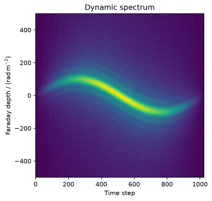
Let’s look at the results

fig, ax = plt.subplots()
ax.imshow(
    np.abs(fdf_spectrum),
    # aspect="auto",
    origin="lower",
    extent=(0, n_times, np.min(phis), np.max(phis)),
)
ax.set(
    xlabel="Time step",
    ylabel=f"Faraday depth / ({u.rad / u.m**2:latex_inline})",
    title="Dynamic spectrum",
)

[Text(0.5, 0, 'Time step'),
 Text(0, 0.5, 'Faraday depth / ($\\mathrm{rad\\,m^{-2}}$)'),
 Text(0.5, 1.0, 'Dynamic spectrum')]

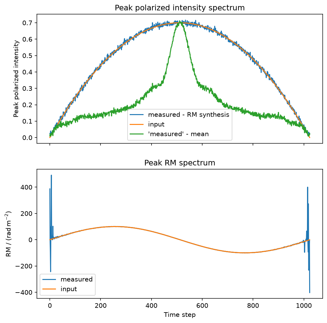
Now let’s recover the PI and RM from the Faraday spectrum. We’ll compare to just taking the mean across frequency. Taking the mean will not perform well due to bandwidth depolarisation.

peak_pi_spectrum = np.max(np.abs(fdf_spectrum), axis=0)
max_pixels = np.argmax(np.abs(fdf_spectrum), axis=0)

peak_rm_spectrum = phis[max_pixels]


## This is the *wrong* thing to do:
stokes_q, stokes_u = np.real(dynamic_spectrum), np.imag(dynamic_spectrum)
stokes_q_mean = np.mean(stokes_q, axis=0)
stokes_u_mean = np.mean(stokes_u, axis=0)
pi_mean = np.hypot(stokes_q_mean, stokes_u_mean)


fig, (ax1, ax2) = plt.subplots(2, 1, sharex=True, figsize=(8, 8))
ax1.plot(time_chan, peak_pi_spectrum, label="measured - RM synthesis")
ax1.plot(time_chan, frac_pol_time, label="input")
ax1.plot(time_chan, pi_mean, label="'measured' - mean")

ax1.legend()

ax2.plot(time_chan, peak_rm_spectrum, label="measured")
ax2.plot(time_chan, rm_time, label="input")
ax2.legend()

ax2.set(
    xlabel="Time step",
    ylabel=f"RM / ({u.rad / u.m**2:latex_inline})",
    title="Peak RM spectrum",
)
ax1.set(
    ylabel="Peak polarized intensity",
    title="Peak polarized intensity spectrum",
)

[Text(0, 0.5, 'Peak polarized intensity'),
 Text(0.5, 1.0, 'Peak polarized intensity spectrum')]