1D RM-synthesis¶

[1]:

from __future__ import annotations

import astropy.units as u
import matplotlib.pyplot as plt
import numpy as np
from astropy.visualization import quantity_support
from numpy.typing import NDArray
from rm_lite.tools_1d import rmsynth

plt.rcParams["figure.dpi"] = 150

_ = quantity_support()
rng = np.random.default_rng(42)

First generate some synthetic data

[2]:

from rm_lite.utils.synthesis import faraday_simple_spectrum, freq_to_lambda2


def faraday_slab_spectrum(
    freq_arr_hz: NDArray[np.float64],
    frac_pol: float,
    psi0_deg: float,
    rm_radm2: float,
    delta_rm_radm2: float,
) -> NDArray[np.complex128]:
    lambda_sq_arr_m2 = freq_to_lambda2(freq_arr_hz)

    return (
        frac_pol
        * np.exp(2j * (np.deg2rad(psi0_deg) + rm_radm2 * lambda_sq_arr_m2))
        * (
            np.sin(delta_rm_radm2 * lambda_sq_arr_m2)
            / (delta_rm_radm2 * lambda_sq_arr_m2)
        )
    )


def faraday_gaussian_spectrum(
    freq_arr_hz: NDArray[np.float64],
    frac_pol: float,
    psi0_deg: float,
    rm_radm2: float,
    sigma_rm_radm2: float,
):
    lambda_sq_arr_m2 = freq_to_lambda2(freq_arr_hz)
    rm_term = np.exp(2j * (np.deg2rad(psi0_deg) + rm_radm2 * lambda_sq_arr_m2))
    depol_term = np.exp(-2.0 * sigma_rm_radm2**2 * lambda_sq_arr_m2**2)
    return frac_pol * rm_term * depol_term

Here we’ll simulate RACS-all frequency coverage

[3]:

bw_low = 288
bw_mid = 144
bw_high = 288
low = np.linspace(943.5 - bw_low / 2, 943.5 + bw_low / 2, 36) * u.MHz
mid = np.linspace(1367.5 - bw_mid / 2, 1367.5 + bw_mid / 2, 9) * u.MHz
high = np.linspace(1655.5 - bw_high / 2, 1655.5 + bw_high / 2, 9) * u.MHz
freqs = np.concatenate([low, mid, high])
freq_hz = freqs.to(u.Hz).value

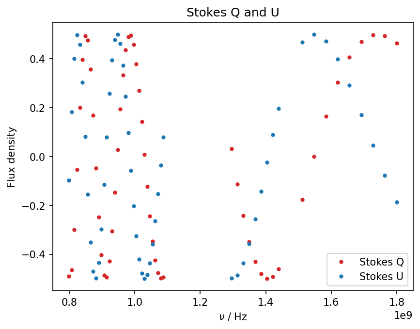
Now we make a Faraday simple spectrum with a single RM component. We will use the following parameters:

[4]:

delta_rm_radm2 = 30
rm_radm2 = 100
frac_pol = 0.5
psi0_deg = 10
complex_data_noiseless = faraday_simple_spectrum(
    freq_arr_hz=freq_hz,
    frac_pol=frac_pol,
    psi0_deg=psi0_deg,
    rm_radm2=rm_radm2,
)

[5]:

fig, ax = plt.subplots()
ax.plot(
    freq_hz, np.real(complex_data_noiseless), ".", label="Stokes Q", color="tab:red"
)
ax.plot(
    freq_hz, np.imag(complex_data_noiseless), ".", label="Stokes U", color="tab:blue"
)
ax.legend()
ax.set(
    xlabel=rf"$\nu$ / {u.Hz:latex_inline}",
    ylabel="Flux density",
    title="Stokes Q and U",
)

[5]:

[Text(0.5, 0, '$\\nu$ / $\\mathrm{Hz}$'),
 Text(0, 0.5, 'Flux density'),
 Text(0.5, 1.0, 'Stokes Q and U')]

Now we can run RM-synthesis by calling rmsynth.run_rmsynth

[6]:

help(rmsynth.run_rmsynth)

Help on function run_rmsynth in module rm_lite.tools_1d.rmsynth:

run_rmsynth(freq_arr_hz: 'NDArray[np.float64]', complex_pol_arr: 'NDArray[np.complex128]', complex_pol_error: 'NDArray[np.complex128]', stokes_i_arr: 'NDArray[np.float64] | None' = None, stokes_i_error_arr: 'NDArray[np.float64] | None' = None, stokes_i_model_arr: 'NDArray[np.float64] | None' = None, stokes_i_model_error: 'NDArray[np.float64] | None' = None, phi_max_radm2: 'float | None' = None, d_phi_radm2: 'float | None' = None, n_samples: 'float | None' = 10.0, weight_type: "Literal['variance', 'uniform']" = 'variance', do_fit_rmsf: 'bool' = False, do_fit_rmsf_real: 'bool' = False, fit_function: "Literal['log', 'linear']" = 'log', fit_order: 'int' = 2, ignore_stokes_i: 'bool' = False) -> 'RMSynth1DResults'
    Run RM-synthesis on 1D data

    Args:
        freq_arr_hz (NDArray[np.float64]): Frequencies in Hz
        complex_pol_arr (NDArray[np.complex128]): Complex polarisation values (Q + iU)
        complex_pol_error (NDArray[np.float64]): Complex polarisation errors (dQ + idU)
        stokes_i_arr (NDArray[np.float64] | None, optional): Total itensity values. Defaults to None.
        stokes_i_error_arr (NDArray[np.float64] | None, optional): Total intensity errors. Defaults to None.
        stokes_i_model_arr (NDArray[np.float64] | None, optional): Total intensity model array. Defaults to None.
        stokes_i_model_error (NDArray[np.float64] | None, optional): Total intensity model error. Defaults to None.
        phi_max_radm2 (float | None, optional): Maximum Faraday depth. Defaults to None.
        d_phi_radm2 (float | None, optional): Spacing in Faraday depth. Defaults to None.
        n_samples (float | None, optional): Number of samples across the RMSF. Defaults to 10.0.
        weight_type ("variance", "uniform", optional): Type of weighting. Defaults to "variance".
        do_fit_rmsf (bool, optional): Fit the RMSF main lobe. Defaults to False.
        do_fit_rmsf_real (bool, optional): The the real part of the RMSF. Defaults to False.
        fit_function ("log" | "linear", optional): _description_. Defaults to "log".
        fit_order (int, optional): Polynomial fit order. Defaults to 2. Negative values will iterate until the fit is good.

    Returns:
        RMSynth1DResults:
            fdf_parameters (pl.DataFrame): FDF parameters
            fdf_arrs (pl.DataFrame): RMSynth arrays
            rmsf_arrs (pl.DataFrame): RMSF arrays

[7]:

fdf_parameters, fdf_arrs, rmsf_arrs, stokes_i_arrs = rmsynth.run_rmsynth(
    freq_arr_hz=freq_hz,
    complex_pol_arr=complex_data_noiseless,
    complex_pol_error=np.zeros_like(complex_data_noiseless),
    do_fit_rmsf=True,
    n_samples=100,
)

WARNING rmsynth.run_rmsynth: Stokes I array/errors or model not provided. No fractional polarization will be calculated.
INFO synthesis.rmsynth_nufft: Running RM-synthesis using the NUFFTs over 2001 Faraday depth channels.
INFO synthesis.rmsynth_nufft: NUFFT complete in 0.00621 seconds.
INFO synthesis.get_rmsf_nufft: Fitting main lobe in each RMSF spectrum.
INFO rmsynth._run_rmsynth: RM-synthesis completed in 16.41ms.

The output values are Polars dataframes that can be inspected easily

[8]:

fdf_parameters

[8]:

shape: (1, 30)

fdf_error_mad	peak_pi_fit	peak_pi_error	peak_pi_fit_debias	peak_pi_fit_snr	peak_pi_fit_index	peak_rm_fit	peak_rm_fit_error	peak_q_fit	peak_u_fit	peak_pa_fit_deg	peak_pa_fit_deg_error	peak_pa0_fit_deg	peak_pa0_fit_deg_error	fit_function	lam_sq_0_m2	ref_freq_hz	fwhm_rmsf_radm2	fdf_error_noise	fdf_q_noise	fdf_u_noise	min_freq_hz	max_freq_hz	n_channels	median_d_freq_hz	frac_pol	frac_pol_error	sigma_add	sigma_add_minus	sigma_add_plus
f64	f64	f64	f64	f64	i64	f64	f64	f64	f64	f64	f64	f64	f64	str	f64	f64	f64	f64	f64	f64	f64	f64	i64	f64	f64	f64	f64	f64	f64
NaN	0.500279	0.0	0.500279	inf	1296	99.999904	0.0	-0.202569	-0.457124	123.050018	0.0	10.000453	0.0	"log"	0.082563	1.0433e9	34.522161	0.0	0.0	0.0	7.995e8	1.7995e9	54	8.2286e6	NaN	NaN	NaN	NaN	NaN

[9]:

fdf_arrs

[9]:

shape: (2_001, 2)

phi_arr_radm2	fdf_dirty_complex_arr
f64	object
-336.725921	(-0.012941228878331957+0.005575863548037922j)
-336.389195	(-0.01358374673356818+0.005189841778274779j)
-336.052469	(-0.014212464149613874+0.004794433774264847j)
-335.715743	(-0.014826491134032707+0.004389815340041808j)
-335.379017	(-0.01542494740046531+0.0039761686503574775j)
…	…
335.379017	(-0.0009008454185260103+0.008053356708390892j)
335.715743	(-0.0009576577337939412+0.00788523016762047j)
336.052469	(-0.0009822777769253547+0.007717713719134412j)
336.389195	(-0.0009751524589895343+0.0075511263409965435j)
336.725921	(-0.0009367729099198278+0.007385776163134531j)

[10]:

rmsf_arrs

[10]:

shape: (4_003, 2)

phi2_arr_radm2	rmsf_complex_arr
f64	object
-673.788568	(-0.03295766077581885-0.03608362753022101j)
-673.451842	(-0.032467191441502584-0.03631484421233953j)
-673.115116	(-0.031940535967829364-0.03653906199687861j)
-672.77839	(-0.03137774876643758-0.03675625231592649j)
-672.441664	(-0.030778933355256957-0.03696638016759515j)
…	…
672.441664	(-0.03077893335567348+0.03696638016745694j)
672.77839	(-0.03137774876682965+0.03675625231578334j)
673.115116	(-0.03194053596819691+0.03653906199673027j)
673.451842	(-0.03246719144184597+0.036314844212186545j)
673.788568	(-0.03295765556151062+0.036083626561931655j)

Since we provided no Stokes \(I\) data, the stokes I model will just be unity with 0 error. The flag_arr array tells us which channels were not used in RM-synthesis or model fitting

[11]:

stokes_i_arrs

[11]:

shape: (54, 7)

freq_arr_hz	lambda_sq_arr_m2	stokes_i_model_arr	stokes_i_model_error	flag_arr	complex_pol_arr	complex_pol_error
f64	f64	f64	f64	bool	object	object
7.995e8	0.140606	null	null	true	(-0.49042944532403415-0.09735994638022451j)	0j
8.0773e8	0.137756	null	null	true	(-0.4654241884816873+0.18270283187778674j)	0j
8.1596e8	0.134992	null	null	true	(-0.3001379571186853+0.3998964949791661j)	0j
8.2419e8	0.13231	null	null	true	(-0.053617325136419355+0.497116870006657j)	0j
8.3241e8	0.129707	null	null	true	(0.20074123829142537+0.45793335240974226j)	0j
…	…	…	…	…	…	…
1.6555e9	0.032793	null	null	true	(0.4056251419940925+0.29234952399871j)	0j
1.6915e9	0.031412	null	null	true	(0.46997598588767076+0.17065336998990638j)	0j
1.7275e9	0.030117	null	null	true	(0.49801253407054746+0.04453668048509923j)	0j
1.7635e9	0.0289	null	null	true	(0.49406601726750204-0.07680345422849415j)	0j
1.7995e9	0.027755	null	null	true	(0.463743096038396-0.1869287053309979j)	0j

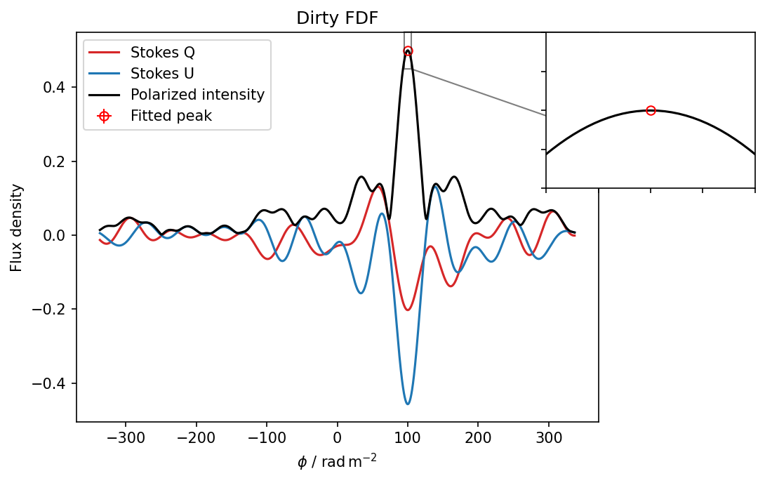
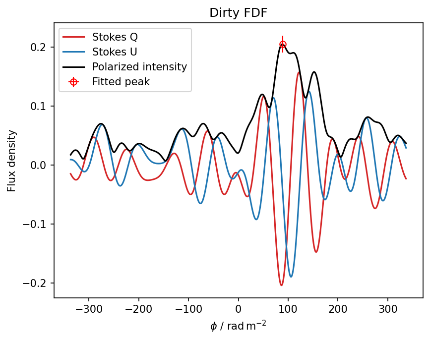
We can also easily visualise the data

[12]:

phi_arr_radm2 = fdf_arrs["phi_arr_radm2"].to_numpy()
fdf_dirty_arr = fdf_arrs["fdf_dirty_complex_arr"].to_numpy().astype(complex)

fig, ax = plt.subplots()
x1, x2, y1, y2 = 95, 105, 0.45, 0.55  # subregion of the original image
axins = ax.inset_axes(
    (0.9, 0.6, 0.4, 0.4), xlim=(x1, x2), ylim=(y1, y2), xticklabels=[], yticklabels=[]
)
for _ax in [ax, axins]:
    _ax.plot(
        phi_arr_radm2,
        fdf_dirty_arr.real,
        color="tab:red",
        label="Stokes Q",
    )
    _ax.plot(
        phi_arr_radm2,
        fdf_dirty_arr.imag,
        color="tab:blue",
        label="Stokes U",
    )
    _ax.plot(
        phi_arr_radm2,
        np.abs(fdf_dirty_arr),
        color="k",
        label="Polarized intensity",
    )

    _ax.errorbar(
        fdf_parameters["peak_rm_fit"],
        fdf_parameters["peak_pi_fit"],
        xerr=fdf_parameters["peak_rm_fit_error"],
        yerr=fdf_parameters["peak_pi_error"],
        fmt="o",
        lw=1,
        color="red",
        mfc="none",
        label="Fitted peak",
    )

ax.set(
    xlabel=rf"$\phi$ / {u.rad / u.m**2:latex_inline}",
    ylabel="Flux density",
    title="Dirty FDF",
    # xlim=[50, 150],
)
ax.indicate_inset_zoom(axins, edgecolor="black")
ax.legend()

[12]:

<matplotlib.legend.Legend at 0x7b9ab239dbe0>

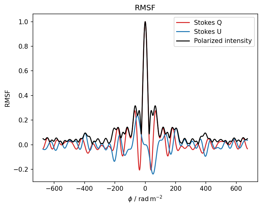
[13]:

phi2_arr_radm2 = rmsf_arrs["phi2_arr_radm2"].to_numpy()
rmsf_arr = rmsf_arrs["rmsf_complex_arr"].to_numpy().astype(complex)

fig, ax = plt.subplots()
ax.plot(
    phi2_arr_radm2,
    rmsf_arr.real,
    color="tab:red",
    label="Stokes Q",
)
ax.plot(
    phi2_arr_radm2,
    rmsf_arr.imag,
    color="tab:blue",
    label="Stokes U",
)
ax.plot(
    phi2_arr_radm2,
    np.abs(rmsf_arr),
    color="k",
    label="Polarized intensity",
)
ax.legend()
ax.set(
    xlabel=rf"$\phi$ / {u.rad / u.m**2:latex_inline}",
    ylabel="RMSF",
    title="RMSF",
)

[13]:

[Text(0.5, 0, '$\\phi$ / $\\mathrm{rad\\,m^{-2}}$'),
 Text(0, 0.5, 'RMSF'),
 Text(0.5, 1.0, 'RMSF')]

Now lets do a more complex example. We’ll add noise and a Stokes \(I\) spectrum

[14]:

from rm_lite.utils.fitting import power_law

[15]:

delta_rm_radm2 = 30
rm_radm2 = 100
frac_pol = 0.5
psi0_deg = 10
complex_data_noiseless = faraday_slab_spectrum(
    freq_arr_hz=freq_hz,
    frac_pol=frac_pol,
    psi0_deg=psi0_deg,
    rm_radm2=rm_radm2,
    delta_rm_radm2=delta_rm_radm2,
)


stokes_i_flux = 1.0
spectral_index = -0.7
rms_noise = 0.1


stokes_i_model = power_law(order=1)
stokes_i_noiseless = stokes_i_model(
    freq_hz / (np.mean(freq_hz)), stokes_i_flux, spectral_index
)
stokes_i_noise = rng.normal(0, rms_noise, size=freq_hz.size)
stokes_i_noisy = stokes_i_noiseless + stokes_i_noise


stokes_q_noise = rng.normal(0, rms_noise, size=freq_hz.size)
stokes_u_noise = rng.normal(0, rms_noise, size=freq_hz.size)
complex_noise = stokes_q_noise + 1j * stokes_u_noise

complex_flux = complex_data_noiseless * stokes_i_noiseless
complex_data_noisy = complex_data_noiseless + complex_noise

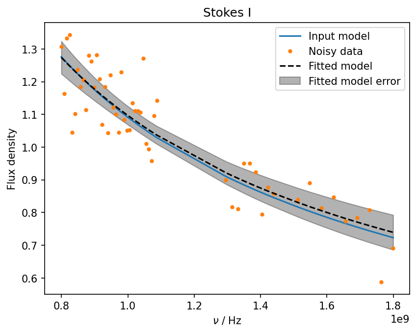
Now we enable Stokes \(I\) model fitting through providing the data, and enabling fit_order. If fit_order<0 an iterative fit will be performed.

[16]:

fdf_parameters, fdf_arrs, rmsf_arrs, stokes_i_arrs = rmsynth.run_rmsynth(
    freq_arr_hz=freq_hz,
    complex_pol_arr=complex_data_noisy,
    complex_pol_error=np.ones_like(complex_data_noiseless)
    * (rms_noise + rms_noise * 1j),
    stokes_i_arr=stokes_i_noisy,
    stokes_i_error_arr=np.ones_like(stokes_i_noisy) * rms_noise,
    do_fit_rmsf=True,
    n_samples=100,
    fit_order=-3,
)

INFO synthesis.create_fractional_spectra: Fitting Stokes I model to calculate fractional spectra.
INFO fitting.dynamic_fit: Iteratively fitting Stokes I model of type log with max order 3.
INFO fitting.static_fit: Fitting Stokes I model of type log with order 0.
INFO fitting.static_fit: Fit results: ['1.04 ± 0.01']
INFO fitting.static_fit: Fitting Stokes I model of type log with order 1.
INFO fitting.static_fit: Fit results: ['1.07 ± 0.01', '-0.67 ± 0.06']
INFO fitting.static_fit: Fitting Stokes I model of type log with order 2.
INFO fitting.static_fit: Fit results: ['1.08 ± 0.02', '-0.62 ± 0.08', '-0.6 ± 0.7']
INFO fitting.static_fit: Fitting Stokes I model of type log with order 3.
INFO fitting.static_fit: Fit results: ['1.08 ± 0.02', '-0.6 ± 0.1', '-1 ± 1', '0 ± 7']
INFO fitting.dynamic_fit: Fit results for orders [0 1 2 3]:
INFO fitting.dynamic_fit: Best fit found with 2 parameters.
INFO synthesis.rmsynth_nufft: Running RM-synthesis using the NUFFTs over 2001 Faraday depth channels.
INFO synthesis.rmsynth_nufft: NUFFT complete in 0.00647 seconds.
INFO synthesis.get_rmsf_nufft: Fitting main lobe in each RMSF spectrum.
INFO rmsynth._run_rmsynth: RM-synthesis completed in 14.28ms.

[17]:

fdf_parameters

[17]:

shape: (1, 30)

fdf_error_mad	peak_pi_fit	peak_pi_error	peak_pi_fit_debias	peak_pi_fit_snr	peak_pi_fit_index	peak_rm_fit	peak_rm_fit_error	peak_q_fit	peak_u_fit	peak_pa_fit_deg	peak_pa_fit_deg_error	peak_pa0_fit_deg	peak_pa0_fit_deg_error	fit_function	lam_sq_0_m2	ref_freq_hz	fwhm_rmsf_radm2	fdf_error_noise	fdf_q_noise	fdf_u_noise	min_freq_hz	max_freq_hz	n_channels	median_d_freq_hz	frac_pol	frac_pol_error	sigma_add	sigma_add_minus	sigma_add_plus
f64	f64	f64	f64	f64	i64	f64	f64	f64	f64	f64	f64	f64	f64	str	f64	f64	f64	f64	f64	f64	f64	f64	i64	f64	f64	f64	f64	f64	f64
NaN	0.204865	0.014593	0.203666	14.03876	1265	89.359859	1.22953	-0.198355	-0.05037	97.12425	2.040628	34.407422	11.812625	"log"	0.082563	1.0433e9	34.522161	0.014593	0.014614	0.014572	7.995e8	1.7995e9	54	8.2286e6	0.191065	0.01369	2.051059	1.583715	2.530761

[18]:

fdf_arrs

[18]:

shape: (2_001, 2)

phi_arr_radm2	fdf_dirty_complex_arr
f64	object
-336.725921	(-0.014731635204135339+0.009358472946699599j)
-336.389195	(-0.01526292392430415+0.009357187561240448j)
-336.052469	(-0.015787097967295292+0.009348266385212791j)
-335.715743	(-0.016303466212415768+0.009331332951215965j)
-335.379017	(-0.016811337092919102+0.009306022158790533j)
…	…
335.379017	(-0.020918871741566387+0.032038020341368045j)
335.715743	(-0.02147110626568857+0.03130936192053694j)
336.052469	(-0.02199920201618622+0.030581887986703346j)
336.389195	(-0.022503012984533322+0.02985683032235221j)
336.725921	(-0.0229824242903409+0.029135402606415964j)

[19]:

stokes_i_arrs

[19]:

shape: (54, 7)

freq_arr_hz	lambda_sq_arr_m2	stokes_i_model_arr	stokes_i_model_error	flag_arr	complex_pol_arr	complex_pol_error
f64	f64	f64	f64	bool	object	object
7.995e8	0.140606	1.274051	0.049751	true	(0.0434179740436972+0.0819041842141131j)	(0.07850810707056659+0.0785549338109777j)
8.0773e8	0.137756	1.265394	0.04819	true	(0.02397116014637071-0.1657338240891809j)	(0.07903207212223327+0.07927844276138749j)
8.1596e8	0.134992	1.256731	0.046652	true	(0.02459878288190812-0.02737741658031438j)	(0.07957676851873773+0.07957801899490526j)
8.2419e8	0.13231	1.248279	0.045493	true	(0.12772878581371183-0.054835889786256246j)	(0.08024546166272928+0.08013525108956521j)
8.3241e8	0.129707	1.23993	0.044057	true	(-0.09817733003759198-0.112586523015026j)	(0.08072511063908873+0.08074885541830505j)
…	…	…	…	…	…	…
1.6555e9	0.032793	0.781946	0.04916	true	(0.5333366680591517+0.4420962574360933j)	(0.13220874865071564+0.1308716236765678j)
1.6915e9	0.031412	0.770735	0.050209	true	(0.4023148966443312+0.12528799561594808j)	(0.13236689230318016+0.13000280209655277j)
1.7275e9	0.030117	0.760002	0.051284	true	(0.5426641976989826-0.10496601738210094j)	(0.13657907272897332+0.13176908025947298j)
1.7635e9	0.0289	0.74961	0.052279	true	(0.45284024924819266-0.2188452740044619j)	(0.13709010832608803+0.13427296298329203j)
1.7995e9	0.027755	0.739467	0.053242	true	(0.5112896286601861-0.32264908513686663j)	(0.14015362580857899+0.1372133772387198j)

[20]:

fig, ax = plt.subplots()
ax.plot(freq_hz, stokes_i_noiseless, label="Input model")
ax.plot(freq_hz, stokes_i_noisy, ".", label="Noisy data")
ax.plot(
    stokes_i_arrs["freq_arr_hz"],
    stokes_i_arrs["stokes_i_model_arr"],
    "k--",
    label="Fitted model",
)
ax.fill_between(
    stokes_i_arrs["freq_arr_hz"],
    stokes_i_arrs["stokes_i_model_arr"] - stokes_i_arrs["stokes_i_model_error"],
    stokes_i_arrs["stokes_i_model_arr"] + stokes_i_arrs["stokes_i_model_error"],
    alpha=0.3,
    color="k",
    label="Fitted model error",
)
ax.legend()
ax.set(
    xlabel=rf"$\nu$ / {u.Hz:latex_inline}",
    ylabel="Flux density",
    title="Stokes I",
)

[20]:

[Text(0.5, 0, '$\\nu$ / $\\mathrm{Hz}$'),
 Text(0, 0.5, 'Flux density'),
 Text(0.5, 1.0, 'Stokes I')]

[21]:

phi_arr_radm2 = fdf_arrs["phi_arr_radm2"].to_numpy()
fdf_dirty_arr = fdf_arrs["fdf_dirty_complex_arr"].to_numpy().astype(complex)

fig, ax = plt.subplots()

ax.plot(
    phi_arr_radm2,
    fdf_dirty_arr.real,
    color="tab:red",
    label="Stokes Q",
)
ax.plot(
    phi_arr_radm2,
    fdf_dirty_arr.imag,
    color="tab:blue",
    label="Stokes U",
)
ax.plot(
    phi_arr_radm2,
    np.abs(fdf_dirty_arr),
    color="k",
    label="Polarized intensity",
)

ax.errorbar(
    fdf_parameters["peak_rm_fit"],
    fdf_parameters["peak_pi_fit"],
    xerr=fdf_parameters["peak_rm_fit_error"],
    yerr=fdf_parameters["peak_pi_error"],
    fmt="o",
    lw=1,
    color="red",
    mfc="none",
    label="Fitted peak",
)

ax.set(
    xlabel=rf"$\phi$ / {u.rad / u.m**2:latex_inline}",
    ylabel="Flux density",
    title="Dirty FDF",
)
ax.legend()

[21]:

<matplotlib.legend.Legend at 0x7b9ab23227b0>

[22]:

phi2_arr_radm2 = rmsf_arrs["phi2_arr_radm2"].to_numpy()
rmsf_arr = rmsf_arrs["rmsf_complex_arr"].to_numpy().astype(complex)

fig, ax = plt.subplots()
ax.plot(
    phi2_arr_radm2,
    rmsf_arr.real,
    color="tab:red",
    label="Stokes Q",
)
ax.plot(
    phi2_arr_radm2,
    rmsf_arr.imag,
    color="tab:blue",
    label="Stokes U",
)
ax.plot(
    phi2_arr_radm2,
    np.abs(rmsf_arr),
    color="k",
    label="Polarized intensity",
)
ax.legend()
ax.set(
    xlabel=rf"$\phi$ / {u.rad / u.m**2:latex_inline}",
    ylabel="RMSF",
    title="RMSF",
)

[22]:

[Text(0.5, 0, '$\\phi$ / $\\mathrm{rad\\,m^{-2}}$'),
 Text(0, 0.5, 'RMSF'),
 Text(0.5, 1.0, 'RMSF')]